[AI Ideas Notebook 02] Timestral: forecast tomorrow's numbers without asking a chatbot to guess
An introduction to Mistral's small time-series models: what probabilistic forecasts mean, where they help, and how to begin with a CPU experiment and an honest comparison.
AI Ideas Notebook explores the ideas and practical possibilities behind newly emerging AI models and tools.
Tomorrow's support queue is a number before it becomes a paragraph. You may want to know whether to assign another person, whether a server needs more capacity, or whether the usual stock order will cover the weekend. A fluent explanation is useful only after the forecast has something solid behind it.
Timestral, introduced by Mistral AI on October 15, 2026, is a family of models for forecasting sequences of numbers. It produces probabilistic predictions rather than chat replies, supports multiple related series, and comes in four published sizes: 5M, 28M, 123M and 209M parameters. Mistral announcement
This introduction takes you from that description to a first useful experiment. We will look at what to feed the model, how to read a forecast range, and how to compare it with a simple baseline. The examples are proposed exercises, so you can try the idea without mistaking an illustration for a measured result.
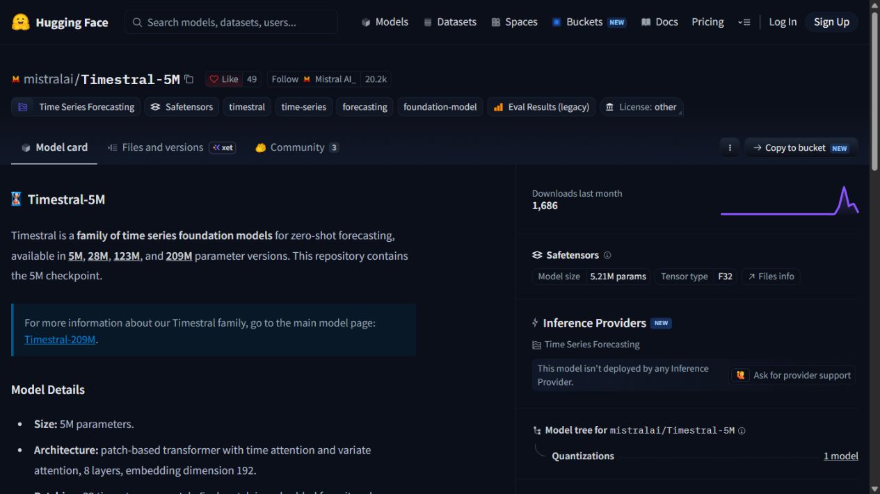 Mistral AI's Timestral-5M page, captured October 20, 2026. The screen identifies a forecasting checkpoint; it is not a chart from an experiment conducted for this article.
A forecast starts with a clock and a quantity
A time series records a quantity over successive time steps. Examples include the number of requests in each minute, orders per day, or temperature at regular intervals. The spacing is part of the meaning: 100 requests per minute and 100 requests per hour describe very different systems.
Before selecting a model, write the decision in one sentence. “Estimate tomorrow's daily support volume so we can plan coverage” is clearer than “find insights in our data.” It specifies the target, the horizon and the action that might change.
Then decide what one observation represents. A support ticket created today and a ticket resolved today are different events. Combining them into one convenient column can obscure the very bottleneck you wanted to understand.
Timestral belongs after this definition. It can process a numerical history, but the team still owns what those numbers mean. A model cannot repair a target that quietly switches from requests to completed jobs halfway through the file.
The useful output is a range you can act on
A point forecast gives you one number. A probabilistic forecast describes several possible levels of the future value, helping you see how much room there is around the central estimate. Timestral's published output includes 21 quantiles per predicted time step. Inference repository
Imagine a planned exercise in which the median forecast for tomorrow is 100 tickets and a higher quantile is 140. These are invented numbers, but they show the decision: ordinary staffing might cover the central estimate, while a backup plan covers a busier day. The forecast is useful because it changes how you prepare.
The quantile is not a promise that reality will stay below a line. You need to check calibration over repeated historical forecasts. If observations exceed a claimed 90th-percentile forecast much more often than expected, that level is not behaving as a reliable planning boundary for your data.
The appropriate boundary also depends on the decision. Running out of stock and holding a little extra stock have different costs. A team may therefore act on a higher quantile than the median, while another task can tolerate a cheaper, less conservative plan.
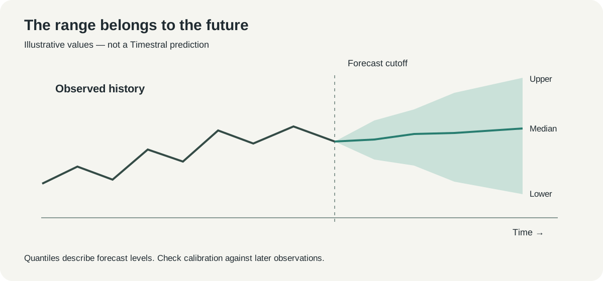 Original explanatory diagram. The curve and range are invented to explain a forecast window; they are not Timestral output.
Related signals help only when their timing is honest
Mistral describes Timestral as a multivariate model with support for past-only and known-future covariates. In everyday terms, it can use several related numerical signals and information whose future values are already available. Release description
A store's opening calendar is known before tomorrow arrives. Tomorrow's actual sales are not. A forecast experiment must respect that difference even when the completed spreadsheet conveniently contains both columns.
For a server-capacity exercise, a scheduled product launch could be known in advance, while the exact request volume remains unknown. For an order-volume exercise, a holiday indicator may be available, while the final number of orders is the target. These are illustrative uses of the distinction, not claims about a deployed integration.
Weather is a useful example of an easy mistake. A historical file may contain the weather that actually happened. A real forecast would have had only the weather prediction available at the time. Evaluating with the later observation gives the system information it would not have had when making the decision.
Start with the smallest experiment that answers a question
The official repository supplies standalone inference on CPU or GPU. A CPU path makes a first test accessible without treating model size as a complete hardware requirement. Dependencies, loaded tensors, history length and the number of series still contribute to runtime memory. Installation and usage
For an introduction, the 5M checkpoint is a reasonable candidate to explore the interface. This is a suggested starting point for a small exercise, not a claim that it will beat larger checkpoints on your data. Establish a working pipeline before comparing model sizes.
- Open the official repository and inspect its installation instructions and license links. Work in a separate Python environment.
- Prepare one regularly sampled series. Keep timestamps and units in your source file even if the numerical array passed to the model contains only values.
- Hold back the last few observations as a test horizon. Do not include them in the history used for that forecast.
- Load a checkpoint, request the chosen horizon, and inspect both the central forecast and the quantiles.
- Compare with a simple forecast made from the same history. Repeat over several earlier cutoffs before drawing a conclusion.
The repository documents this installation route, with Python 3.10 or newer and PyTorch 2.4 or newer as its stated requirements. Installation fetches code; review and pin a revision when you need a reproducible environment.
python -m venv .venv
# Activate the environment using your shell's activation command.
python -m pip install "git+https://github.com/mistralai/timestral.git"
Here is a deliberately small adaptation of the documented inference interface. The values are synthetic daily counts; the code does not imply that this article executed the model or obtained a particular result.
import numpy as np
from timestral import TimestralForecaster

history = np.array([
    80, 83, 85, 88, 96, 61, 58,
    82, 84, 87, 91, 99, 64, 60,
    85, 86, 89, 94, 102, 66, 63,
], dtype=np.float32)

model = TimestralForecaster.from_pretrained("mistralai/Timestral-5M")
forecast = model.forecast(history, prediction_length=7)
print(forecast.median)
print(forecast.quantile(0.9))
Three weeks of invented data are enough to illustrate the API, not enough to establish performance on a business process. Replace them with a suitably long, well-understood series before making a decision. Check missing observations and unusual events rather than quietly turning every gap into zero.
Three jobs show why forecasting differs from text generation
Daily support planning connects a forecast to staffing. The input might be a history of tickets created each day, with a calendar indicating weekends and known closures. The review question is whether the forecast helps prepare capacity, especially for busier days that a simple average misses.
Server planning connects a forecast to a technical limit. Requests per interval may be the target, but errors, latency and accepted capacity still need separate monitoring. A forecast of expected demand cannot establish that an application will survive a particular load.
Stock planning connects a forecast to lead time. If replenishment takes several days, tomorrow's demand alone is the wrong horizon. The useful exercise predicts over the interval in which the next order cannot yet arrive and compares the consequences of shortages and excess stock.
All three examples share a pattern: define the quantity, define when the decision is made, and define what changes because of the forecast. The model then becomes an instrument inside the workflow. It is easier to assess that instrument when the intended action is visible.
Compare forecasts at the moment they could have been made
A backtest recreates earlier forecast opportunities. Pick a historical cutoff, provide only the information available before it, and predict the next interval. Move the cutoff forward and repeat without letting future observations leak backward into model selection.
Start with a baseline that matches the pattern. Last week's value for the same weekday can be useful for a weekly cycle; the most recent value can be useful for a stable short-horizon process. Neither is automatically strong, but both tell you whether added complexity earns its place.
| Comparison | What to hold fixed | What the result can tell you |
|---|---|---|
| Timestral versus a seasonal baseline | Target, cutoffs and forecast horizon | Whether the model improves the decision-relevant errors |
| 5M versus a larger checkpoint | Data preparation and scoring | Whether extra model resources bring enough benefit |
| With and without a known calendar | Historical information available at each cutoff | Whether the extra signal helps without leaking the future |
| Median versus a higher decision quantile | Forecasts and business cost assumptions | How the planning policy changes, rather than how the model changes |
Keep zero and near-zero periods in view. A percentage error can become difficult to interpret when the target is tiny. Use metrics appropriate to the series and inspect the actual misses alongside the aggregate score.
For a practical pilot, a small table of the worst misses often teaches more than one headline average. Was the error associated with a missing interval, a holiday, a system outage, or a real change in demand? The answer determines whether to improve the data pipeline, add information, or reconsider the forecasting approach.
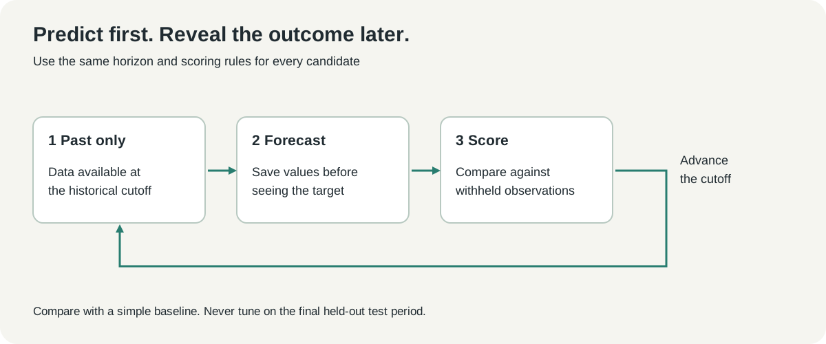 Original backtesting diagram. Every forecast uses information available at its own cutoff; later observations are reserved for scoring.
Small weights are only one part of deployment
The repository distinguishes Apache 2.0 code from model weights released under a Modified MIT license. Read the actual weight terms for the checkpoint you choose; an open repository and a separately licensed model are different distribution artifacts. Repository license explanation
Initial downloads and normal inference are also different stages. The documented loader can use a cached local model, but an application remains offline only when all of its components do. A local forecasting model does not prevent another part of the workflow from sending data to a remote service.
For repeated operation, record which checkpoint produced each forecast and when the input data stopped. A chart without that cutoff can be mistaken for a forecast even when it incorporates later observations. Keep the predicted values unchanged so you can later compare them with what happened.
A forecast service should also have a plan for missing data and failed runs. Showing yesterday's prediction as though it were fresh creates a misleadingly healthy interface. Make the last successful data timestamp visible, and decide when a simple baseline is preferable to a stale model output.
A faster prediction is useful only if the decision improves
Mistral reports CPU-friendly inference and strong benchmark results for the family. Those are reasons to investigate, rather than measurements of your own data pipeline. A published model timing does not include every possible file read, feature calculation, queue or chart in an application. October 15 announcement
There is a common temptation to make the pilot about the largest checkpoint that can run. A better question is whether the forecast arrives before the decision and improves the errors that matter. A somewhat more accurate result delivered after a staffing deadline has limited operational value.
You should also distinguish a numerical improvement from a policy improvement. A lower average error may leave the most costly busy days unchanged. Conversely, a better-calibrated upper quantile may improve planning even when the median moves only slightly.
Decide these criteria before comparing models. The pilot can then end with a useful choice: keep the baseline, use a small checkpoint, or justify a more demanding configuration. Each can be the right outcome when its evidence is clear.
The forecast should leave a record before tomorrow arrives
Our view is that Timestral is interesting because it brings a specialized numerical task into an accessible model workflow. Its output can serve as a weather forecast for a workload: a central expectation, a range, and a reason to prepare. The value appears when those predictions meet a real planning decision.
Begin with one quantity and one horizon. Save the forecast before the outcome is known, then compare it honestly with a simple alternative. That turns a promising model release into an experiment whose result you can actually use.
Sources and media
Checked October 20, 2026. Examples and charts are illustrative, not model execution results. The public model-card screenshot was captured by the author; the explanatory diagrams are original. See the media record for sources and license notices.
- Mistral announcement, October 15, 2026
- Official inference code, installation and license distinction
- Timestral-5M checkpoint
- Checkpoint license
Keep the prediction and the outcome together
Save the data definition, forecast cutoff and review notes alongside the original source links. Telli.sh can help organize that experiment record. Create a Telli.sh account